Automatic Polynomial Form Correction with Autocorrelation Functions¶
Table Of Content
Foreword
The following study has been undertaken during a PhD work funded by ArcelorMittal Research and completed at Mines ParisTech ARMINES. Its recollection in the present form intends to publicize a method designed to solve a pratical measurement problem, and can also be considered as a translation of the corresponding chapter of the PhD thesis [Nion2008].
Abstract
Dealing with a surface’s form is an essential part of any topographical study of the said surface’s roughness. We present here a method for automatic correction of the form, using very simple concepts to solve a problem where top notch technologies were not enough mature to tackle. After explaining how well known mathematical tools such as the correlation function relate to this problem, we will see how they helped us to design an automatic procedure that we applied in order to get a highly reliable data set, that, in turn, underpinned a fine grain study on rough surfaces conducted at ArcelorMittal Research.
Keywords: surface, form, roughness, correlation, modelisation
Introduction¶
When conducting experiments on surfaces with expected changes of topographies according to some process (like wear, painting, etc.), and when these evolutions are the main subject of interest, it is crucial to be able to accurately measure the topography in a reproducible and artifact-free manner.
A well known artifact, omnipresent in surface studies, is the form (also called form factor) whose morphology can hardly be characterised precisely and whose existence is usually more related with the experimental protocol than with the actual physical phenomena of interest. Hence, many topographical studies require a correction of the surfaces’ forms; a correction which is very often hand-made and thus induces an obvious lack of reproducibility.
These sources of inaccuracy were identified as a major obstacle to the fulfilment of a PhD project [Nion2008] started in collaboration between the Center for Mathematical Morphology (Mines ParisTech) and ArcelorMittal Research. Our main purpose was then to investigate the way paint could interact with a steel sheet’s topography during the coating process. This kind of study requires the highest precision in the input data since the physical phenomena take place at a wide range of scales – including the tiniest ones. Moreover, the evolution of the topography of a given surface was our main interest, hence we had to ensure the highest level of reproducibility during our experimental data acquisition, in order to be able to analyse the correct evolution at each point of the surface during the painting process.
In the following, we will see how this was achieved by introducing the most basic tools we used in a first manual approach to form correction. Then we will recall a few facts about the correlation function that helped us automatise the whole process. This will naturally lead us to the description of the automatic process itself and its results. Eventually, we will propose some concluding remarks and pinpoint the possible ways of improvement to our technique.
A simple correction method¶
The measure of a surface’s topography is commonly interpreted as the sum of three main components of increasing typical scales: roughness, waviness, and form. This classification naturally led researchers to favour the use of multiscale filters, when looking for characterisation or correction of the form. Hence Gaussian based methods were first developed that are nowadays replaced by various evolutions of the wavelet tools like the continuous wavelets proposed by Zahaounai [Zahouani2001] and Lee [Lee1998] and the complex wavelet proposed by Jiang et al [Jiang2004]. A good review of these tools, their applications and evolutions, and can be found in [Mezghani2005phd] and [Jiang2007]. Though we are not questioning the performances of these advanced tools, we have chosen to base our method on much simpler ones for reasons that we will now explain.
Our approach to deal with form correction was inspired by the manual correction method that was already used in ArcelorMital Research’s labs for 1-D profiles. The method consists in searching a description of the form by fitting a polynomial curve to the measured profile. This is clearly an application of the familiar definition of the best-fit line defined in surfaces metrology [Whitehouse1994]. As the method produced acceptable results for profiles, we settled on trying to extend it to the two dimensional case and then to make it automatic.
Following this track implies that we formally assume that the form of a surface can be modelled by a polynomial surface. And the core algorithm in our method is indeed a trial and error approach that starts by fitting a polynomial surface of a fixed degree [*] to the measured topography, and by correcting this topography by the fitted polynomial. Then, if the correction is judged to be insuficient, we try to fit a polynomial surface with an increased degree, and so on until the correction is satisfactory. The fit is performed by a least square method, and, for this first version of the algorithm the quality of the fit is simply evaluated by the user, looking at the corrected surface.
The extreme simplicity of this method should not be judged too lightly though. Actually, this is a first step towards what allowed us to find an automatic form correction algorithm as we will see in the next sections. But it also gave us easy ways to optimise the process and make it industrially usable. One of the major challenges we faced was that our images were quite large (each topography being described by an array of approx. 7000x4000 real valued points), and required important computational resources even for a simple least-square fitting. However by leveraging our first assumption that we could describe the form by a simple polynomial model – defined on a continuous space – but also taking into account the fact that we are interested in a feature that has a large typical scale compared to the rest of the features of a surface, we could perform the least-square fit on a subsampled topography. So, for the whole process, the fit was performed on an image of the size a hundredth of the original size, and only the form subtraction was performed on the real-size image.
This simple subsampling saved a lot of time, but it could also be argued that it can cause severe damage and make us fall in the well known defect of fitting polynomials on a finite set of point, that is that the polynomial is left uncontrolled in between the points – where it can show arbitrarily big “ondulations”. But, due to the fact that we fixed the polynomial’s maximum degree for each fit and by the nature of our step-by-step trial-and-error approach, we ended up fitting polynomial surfaces with reasonably low degrees (up to 10 at most, in practice) on a set of several hundreds of points. This proved to give us good enough form corrections that still needed to be automatised, though.
Enters the correlation function¶
In order to achieve our automatisation goal, we decided to look at the most important point of the process that was defeating this purpose. Considering the description made in the former section, this target appears to be the decision to be taken on the quality of the correction, before choosing to stop the iteration or to try to fit another polynomial. Our main purpose here, will then be to understand how we can quantify the conformity of the tentatively corrected surface with what an expert would call a form-corrected surface.
To explain the difference between a surface in need of further form correction and an adequately corrected surface, experts point at the disappearance of large scale patterns in the spatial arrangement of the corrected topography. Our automatisation process is sticking to this observations up to the point that, while analysing the patterns of a surface’s topography, we won’t concentrate on what the form precisely is, but, instead, we will only characterize the absence of form. Considering the trial-and-error process described in the previous section, the construction of such an absence detector is all you need to define the stopping condition.
To understand how effective criteria can be built, it is necessary to follow a path akin to the already mentioned multiscale approaches in form characterisation. And as a foundation for the rest of our explanation we will adopt the following definition of the form: we will call the form of a topography, a model surface that accounts for all the patterns of the initial topography, whose characteristic lengths are above a certain threshold value [†].
[*] Two remarks can already be given about the above definition. First, the usual definition of the form is respected since we consider that the form accounts for the patterns of highest scales. Second, we do not give a precise value for the threshold scale nor a way to find it, and this is intentional. In practice, the form problem is dependent on the process that produced the surface but also on the process that is intended to be applied on the form-corrected topography of this same surface. Hence a certain degree of freedom that we want to keep in the definition of the threshold.
To use the proposed definition, we decided to use the correlation
function, that is widely used for scale-based characterisations of a
signal’s patterns. We recall below the autocorrelation formula
expressed for a second order stationnary series  where
where
 is the expectation and
  the variance. Since we
will only use here one-dimensional measures of the autorcorrelation on
the topographies, the later can be considered as collections of
discrete series (and for implementation detail on can refer to
[NionAutocorr]).
the variance. Since we
will only use here one-dimensional measures of the autorcorrelation on
the topographies, the later can be considered as collections of
discrete series (and for implementation detail on can refer to
[NionAutocorr]).
![autocorr_f(i,j) = \frac{E\left[ (f_i-\mu)(f_j-\mu) \right]}{var(f)}](_images/math/a5c69876103a50f0ab6b3388e939cbc74c7da97c.png)
As the topographies of the surfaces we have dealt with were quite complex – with a lot of patterns of various scales – we were interested in the behaviour of the correlation function in such a combination of various textures. Fig.: Examples of patterns shows what happens when synthetic patterns with two different scales are mixed (via a simple addition) into a new synthetic topography.
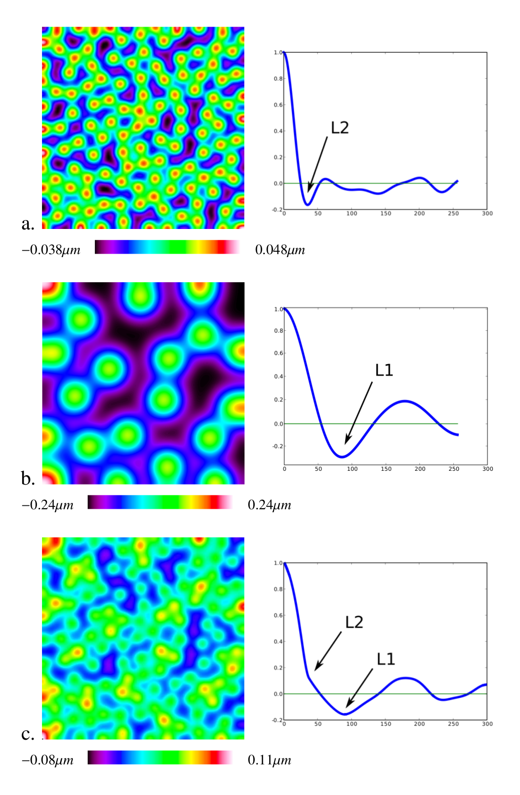
Fig.: Examples of patterns with various scales and their correlation functions.
What is of interest in this example and which we actually used in our method, is the fact that the long-distance correlation, characteristic of the initial large scale pattern, contributes to the combined correlation by shifting to the right the point where the curve crosses the scale axis, and also by “vertically” pulling the curve away from this same scale axis. All said in a much simpler way, the correlations present in the large-scale pattern, is still present and detectable in the correlation function of the combined image. This is very much expected of course, but the little bit over-detailed description we have just made of this phenomenon is exactly what we implemented in order to define our form detection criteria.
We can now discuss the criteria themselves. All of them apply to a 1-d
profile of the correlation function (an apparent simplification which
will be discussed in section Automatisation). The main criterion is
illustrated by Fig.: Form detection criteria-a and requires the
definition of the typical length  above which a pattern is to
be considered as the shape. We can then look at the domain defined by
above which a pattern is to
be considered as the shape. We can then look at the domain defined by
 , for the correlation function, and if the curve does
not cross the scale axis twice on this domain then we can infer that
something is introducing a large-scale correlation in the topography,
and, by definition, this “something” is considered as being part of
the form.
, for the correlation function, and if the curve does
not cross the scale axis twice on this domain then we can infer that
something is introducing a large-scale correlation in the topography,
and, by definition, this “something” is considered as being part of
the form.
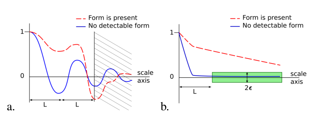
Fig.: Form detection criteria on correlation functions.
However the latest criterion alone does not account for all the cases
when the form is present. For instance if the form-affected topography
also shows a very strong short-scale correlation (e.g. if it bears
some small periodic patterns), it may change its sign more than twice
before the threshold length. Basically this is because the first sign
changes may not be the first to look for and the interval between two
changes is also typical of the scales in presence. However to take
this into account, we choose to perform a mean-filter on the
correlation function with a kernel of size  that needs
to be chosen accordingly with the nature of the study (as is the
threshold length). This approximation makes our first criterion to
cover most of the cases we’ve encountered.
that needs
to be chosen accordingly with the nature of the study (as is the
threshold length). This approximation makes our first criterion to
cover most of the cases we’ve encountered.
A second criterion is however needed, for the very specific case when
the surface hardly shows any pattern apart from its form, which
happens when dealing with a polished surface – where the patterns
usually are of smaller size than the sampling step used for the
measure. To detect this absence of small to medium scales
correlations, we propose the criterion described by Fig.: Form
detection criteria-b where we reuse the threshold scale defined
above and where we introduce a new parameter  that
makes it possible to define a cylinder around the scale axis, starting
at scale , extending to infinity and with a base-radius of
. We then decide that if the curve is inside the
cylinder at scale , and stays in it “forever” [‡] then it
has definitely no form. Interestingly, designing this criterion gave
us the idea to use the same kind of cylinder to help make the first
criterion even more robust to signal noises by detecting a sign change
only when the curve crossed a cylinder of base-radius
that
makes it possible to define a cylinder around the scale axis, starting
at scale , extending to infinity and with a base-radius of
. We then decide that if the curve is inside the
cylinder at scale , and stays in it “forever” [‡] then it
has definitely no form. Interestingly, designing this criterion gave
us the idea to use the same kind of cylinder to help make the first
criterion even more robust to signal noises by detecting a sign change
only when the curve crossed a cylinder of base-radius  .
.
We have now ended up with two criteria that make it possible to
determine if some form is present or not, knowing that each one
applies exclusively to a specific case. Though based on very simple
ideas, they require, in practice, exactly 4 parameters: the first
criterion, that will be referred to as the sign change criterion
requires 3 ( ), and the second one, referred
to as the decorrelation criterion, requires 2 (the same
and ), which can be judged as being too much. We will see
in the next section that these parameters can safely be reduced to two
parameters only.
), and the second one, referred
to as the decorrelation criterion, requires 2 (the same
and ), which can be judged as being too much. We will see
in the next section that these parameters can safely be reduced to two
parameters only.
Automatisation¶
Before describing the automatised process, let’s recall the big picture about the two main tools we will use. On the one hand, the shape correction itself consists in fitting, and then subtracting, a polynomial surface to the measured topography. Besides the least square fitting method, the polynomial is further constrained by only one parameter: the maximum degree of its terms. On the other hand, we use a 1-d profile of the correlation function of a topography to detect the disappearance of the form.
The fact that both the parametrisation of the shape correction and the measure of its quality are one dimensional, makes it possible to build the following simple process described in Automatic form correction algorithm.
measured topography.
form-corrected topography.

(1)
While(FormIsPresent)
(2)

(3)

Automatic form correction
In the algorithm, at point (1), we find the fact that most of the work is done at subresolution, more precisely we create a subresolved copy of the measured topography, from which we select one point out of ten along the scale axis of the topography and one out of ten along the y-axis, which gives us a sub-sampled topography a hundred times smaller than the initial one.
At point (2), we create the polynomial surface. The fit
is made with a least square method (as already explained in A simple
correction method), and we add the constraint that the polynomial
must have no term of degree higher than  . What’s
important to note here is that the function returns an algebraic
description of the polynomial which will be able to adapt to data of
any size (i.e. taking into account the changes in resolution).
. What’s
important to note here is that the function returns an algebraic
description of the polynomial which will be able to adapt to data of
any size (i.e. taking into account the changes in resolution).
Finally, the presence of the form is detected at point
(3), thanks to a function depending on only three
parameters: the surface to be tested, the threshold length
and a tolerance parameter . This is less than expected
from Enters the correlation function, because, in practice, the
then described criteria have proved to be robust to some significant
variations of their parameters, which we interpreted as some freedom
in the algorithm’s parametrisation and that we used in order to reduce
the number of needed parameters.
For instance the sign change criterion is not very sensitive to the
exact value of the parameter, except that it must not
be too small (else it would have no effect), nor too big compared to
(else it would perturbate the criterion and shift the
required threshold scale), so we took it equal to  . Along
the same idea, the parameter, which helps in making the
zero-crossing detection more robust, has the main constraint not to be
equal to zero of course, and to be small below 1 (the maximum value of
the correlation function). It was then safe to chose the value of
. Along
the same idea, the parameter, which helps in making the
zero-crossing detection more robust, has the main constraint not to be
equal to zero of course, and to be small below 1 (the maximum value of
the correlation function). It was then safe to chose the value of
 (
( being the parameter of the
decorrelation criterion).
being the parameter of the
decorrelation criterion).
One more practical fact is worth noting here. We have already mentioned that our criteria were applied on a 1-d profile of the correlation function. Since we are working on 2-d topographies, on which we can naturally compute 2-d correlation functions, the choice of the profile is worth questioning. The steel sheet samples we dealt with had undergone the rolling process, had been cut out of production samples to be painted and baked. Every one of these steps added its lot of constraints and hence contributed to the surface’s deformations, generally along all the directions of the plane, though the rolling direction is known to get more than its due. On our rectangular samples, we chose the largest dimension – that corresponded to the rolling direction – to compute a 1-d correlation: being the largest, it gave the highest a priori probability of showing any form, and being the rolling direction made this probability even higher.
Now that the mechanisms and parametrisation of the algorithm have been exposed, we can have a look at how it performed on the example provided in figure Fig.: Form correction on the topography of a sealer coated steel sheet, where the sign change criterion was the first to detect the disappearance of the form. Interestingly enough, the polynomial degree at which the search for a good correction stopped seemed to vary a lot but to be bounded to low values. Actually, the attentive reader would have noted that the described algorithm does not offer a strong guaranty that it will stop, and in our implementation a limit has been hardcoded to prevent an infinite loop. However the limit (a polynomial degree of 10) was never reached on our data set.
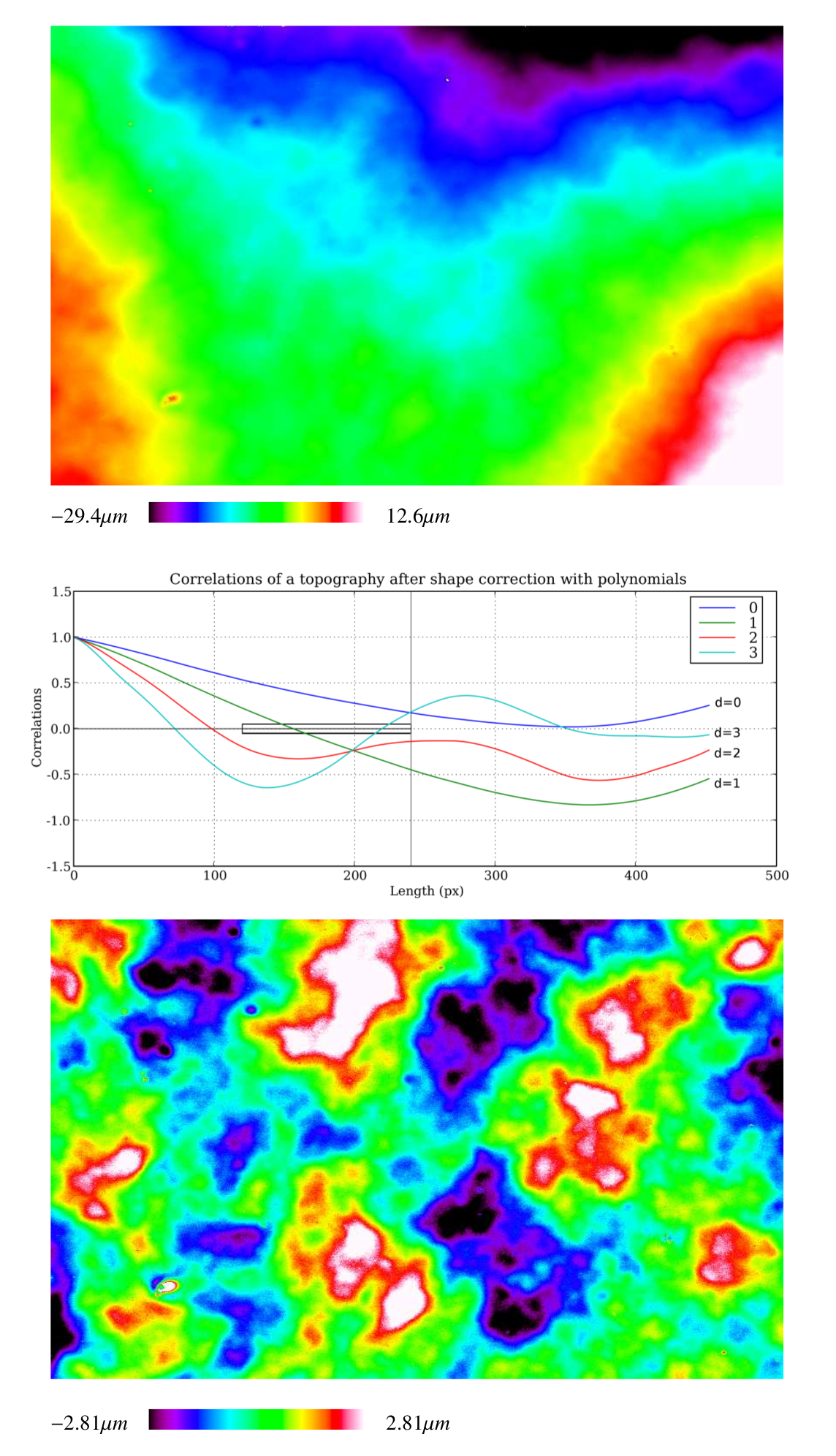
Fig.: Form correction on the topography of a sealer coated steel sheet.
This same algorithm has been applied to 165 topographies, each one being broadly of the same size (7000x4000 pixels). It has been implemented with the Morph-M library [CMM:MorphM] and, when executed on a Linux operated PC with a 3 GHz CPU, 2Gb of RAM, the algorithm took about 5 minutes to generate a fully corrected topography. This time should be judged over the fact that no actual optimisation was made on the image processing operations and that the initial manual correction task is more difficult that letting the machine run, and can be much longer for an less experienced user. The 165 corrected samples were checked by experts from ArcelorMittal’s lab.
After this first validation, our algorithm was integrated in a
standalone programm and transfered to their lab in order to be used in
subsequent projects. A second validation study was later conducted
there [Berrini2008] and revealed a good stability of the
results relative to changes in the sampling scale. It also highlighted
the strong influence the typical length () parameter has on
the selected polynomial degree, both of them being related by a
step-wise decreasing function, where the steps tend to indicate that
there were domains inside which  of will
induce the same selected degree. Such behaviours are good clues that
on top of solving our initial problem, our algorithm is appropriate
for industrial use.
of will
induce the same selected degree. Such behaviours are good clues that
on top of solving our initial problem, our algorithm is appropriate
for industrial use.
Try it!¶
Since the validation was done as an in-house process and mostly on confidential data, we provide a re-implementation of the same algorithm as a pure-Python script.
The scripts are provided in the shape_correction_scripts.zip file
And, while keeping in mind that the algorithm was designed for a very specific kind of data, we give, in this section three examples, quite far from the original scope, but where the effects and limits of the algorithm are visible.
Please note that in the following examples we used a same value for
‘epsilon’ ( ) and that the ‘typical length’
() of the form factor changed from an image to another but
was systematically taken as equal to 2/3 of the images’ longest
side. The range of degrees allowed spanned from 0 to 10.
) and that the ‘typical length’
() of the form factor changed from an image to another but
was systematically taken as equal to 2/3 of the images’ longest
side. The range of degrees allowed spanned from 0 to 10.
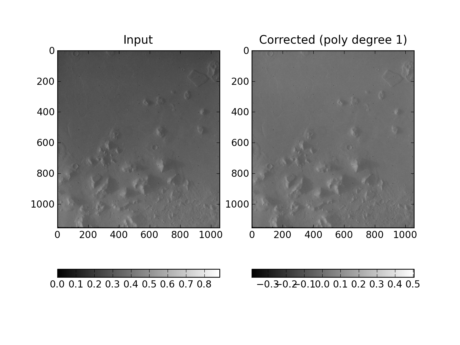
Fig.: Shape correction on a photo of Mars’ surface taken by Viking2.
The form factor to be corrected here is the visible slope spanning from the upper border of the image to the lower one. The algorithm actually found that a polynomial of the 1st degree was enough for the correction. As a downside, one must note that the algorithm does not take illumination effects (e.g. shadows) into account.
Image from NASA ( http://nssdc.gsfc.nasa.gov/photo_gallery/photogallery-mars.html )
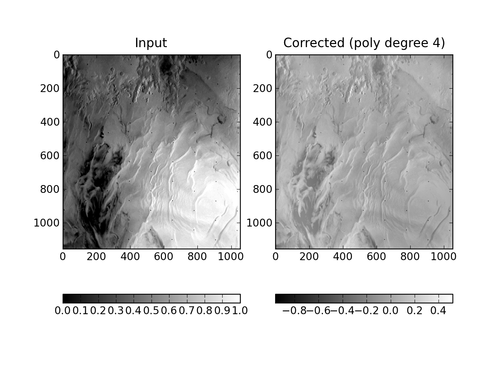
Fig.: Shape correction on another photo of Mars’ surface taken by Viking2.
The form factor to be corrected here is more complex to describe than in the previous example and the algorithm went as far as fitting a 4rth degree polynomial.
Image from NASA ( http://nssdc.gsfc.nasa.gov/photo_gallery/photogallery-mars.html )
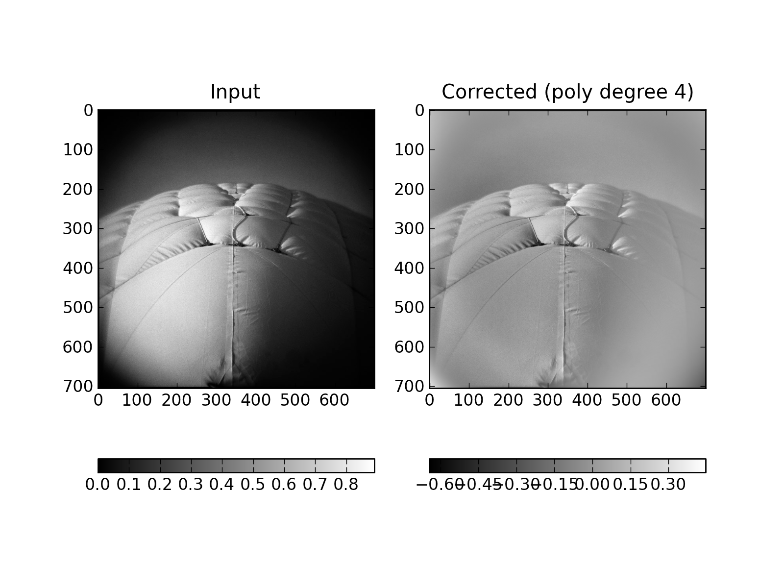
Fig.: Shape correction on a vignetted black and white picture.
Here the algorithm indeed tries to correct the shape but the result is less than convicing. When looking at the details it appears that the shape of the center object has a typical size close to the one of the vignetting effect, which lured the algorithm in trying to correct the ‘inflated’ look of the central object at the same time as the vignetting effect...
Picture taken by photographer: Joe Lencioni (licence CC-by-sa) ( http://en.wikipedia.org/wiki/File:Swanson_tennis_center.jpg )
The three input images corresponding to the previous examples, as well as some illustrations of the intermediate steps are available in the following zip file: shape_correction_examples.zip
Conclusion¶
We have shown here how the understanding of existing processes, like the form correction by polynomials made by quality control experts, and of well known measuring tools like the correlation function, could lead to the design of a fully automatised process aiming at improving the reproducibility of the experiments, and make it industrially viable to exploit large data set.
Our proposed method, though based on simple ideas, has given good enough results: after validation by the experts from ArcelorMittal Research, we made it into a single purpose GUI application for form correction to be used inside ArcelorMittal’s labs to automatise as much as possible of their measurement processes.
Despite this first success, there is of course some place for improvements, mostly to ensure that it may be applicable to other kind of data than steel sheets topography. Such improvements can be expected in the replacement of the polynomial interpolation and subtraction by a more modern method like one based on B-splines or more generally on wavelets that may offer better fitting at a given scale.
It is important, though, to keep in mind that one of the bases of our method is to avoid defining the scale of the form, but instead to define the scale above which a pattern is considered as the form, which may not be that easy to translate in the language of wavelets decomposition for instance. A more promising role for the wavelet would certainly be the enhancement of the form detection that we perform here with a 1-d correlation.
The simplicity and robustness of our basic tools made the strength of our automatic process, and its applicability in several industrial projects.
References¶
| [Nion2008] | (1, 2) T. Nion, Modélisation mathématique de l’évolution de la topographie des couches successives des surfaces peintes destinées au secteur automobile., Ph.D. thesis, École des Mines de Paris – ParisTech. École doctorale: Information, Communication, Modelisation et Simulation (num. 431), 2008. http://pastel.archives-ouvertes.fr/pastel-00626728 |
| [Lee1998] | S.H. Lee, H. Zahouani, R. Caterini, T. G. Mathia. Int. J. Mach. Tools and Manufacturing} vol. 38. 581–589. 1998. |
| [Zahouani2001] | H. Zahouani, S. H. Lee, R. Vargiolu, J. Rousseau. Acta Physica Superficierum, vol. 4. 1–13. 2001. |
| [Jiang2004] |
|
| [Mezghani2005phd] | S. Mezghani. Approches multi-échelles de caractérisation tridimensionnelle des surfaces. Applications aux procédés d’usinage. Ph.D. thesis, École Centrale de Lyon. École Doctorale Mécanique, Energétique, Génie civil et Acoustique (MEGA). 2005. |
| [Jiang2007] | X. Jiang, P. J. Scott, D. J. Whitehouse, L. Blunt. Proc. R. Soc. 2071–2099. 2007. |
| [Whitehouse1994] | D. J. Whitehouse. Handbook of surface metrology, CRC Press, Bristol, UK; Philadelphia, PA: Institue of Physics. 1994. |
| [CMM:MorphM] | CMM/Ecole des Mines/ARMINES/TRANSVALOR, Morph-M: morphological image processing library. 2007. http://cmm.ensmp.fr/Morph-M/ |
| [Berrini2008] | F. Berrini. Rapport de stage en License professionnelle AQI (Acquisition de données, Qualification d’appareillages en milieu industriel). Technical Report. Arcelor Research Automotive Products. 2008. |
| [NionAutocorr] | Thibauld Nion. Autocorrelation functions. http://www.tibonihoo.net/literate_musing/autocorrelations.html |
—
| [*] | The very first try is made with a polynomial of degree 0 just to be sure not to force a correction on a surface that does not need it. |
| [†] | The expression characteristic length is to be understood as the main length parameter that best describes the spatial arrangement of a pattern. For a sinusoidal curve, that would be its period for instance. |
| [‡] | In practice the cylinder has a finite length of so that it
stops at scale  as in our first criterion. as in our first criterion. |